## Practical session: Linear regression
## Jean-Philippe.Vert@mines.org
##
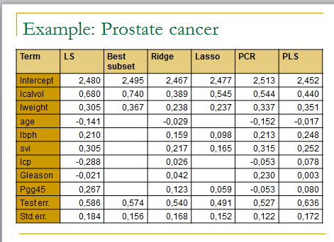
## In this practical session to test several linear regression methods on the prostate cancer dataset
##
####################################
## Prepare data
####################################
# Download prostate data
con = url (“http://www-stat.stanford.edu/~tibs/ElemStatLearn/datasets/prostate.data”)
prost=read.csv(con,row.names=1,sep=”\t”)
# Alternatively, load the file and read from local file as follows
# prost=read.csv(‘prostate.data.txt’,row.names=1,sep=”\t”)
# Scale data and prepare train/test split
prost.std <- data.frame(cbind(scale(prost[,1:8]),prost$lpsa))
names(prost.std)[9] <- ‘lpsa’
data.train <- prost.std[prost$train,]
data.test <- prost.std[!prost$train,]
y.test <- data.test$lpsa
n.train <- nrow(data.train)
####################################
## Ordinary least squares
####################################
m.ols <- lm(lpsa ~ . , data=data.train)
summary(m.ols)
y.pred.ols <- predict(m.ols,data.test)
summary((y.pred.ols – y.test)^2)
# the importance of a feature depends on other features. Compare the following. Explain (visualize).
summary(lm(lpsa~svi,data=datatrain))
summary(lm(lpsa~svi+lcavol,data=datatrain))
####################################
## Best subset selection
####################################
library(leaps)
l <- leaps(data.train[,1:8],data.train[,9],method=’r2′)
plot(l$size,l$r2)
l <- leaps(data.train[,1:8],data.train[,9],method=’Cp’)
plot(l$size,l$Cp)
# Select best model according to Cp
bestfeat <- l$which[which.min(l$Cp),]
# Train and test the model on the best subset
m.bestsubset <- lm(lpsa ~ .,data=data.train[,bestfeat])
summary(m.bestsubset)
y.pred.bestsubset <- predict(m.bestsubset,data.test[,bestfeat])
summary((y.pred.bestsubset – y.test)^2)
####################################
## Greedy subset selection
####################################
library(MASS)
# Forward selection
m.init <- lm(lpsa ~ 1 , data=data.train)
m.forward <- stepAIC(m.init, scope=list(upper=~lcavol+lweight+age+lbph+svi+lcp+gleason+pgg45,lower=~1) , direction=”forward”)
y.pred.forward <- predict(m.forward,data.test)
summary((y.pred.forward – y.test)^2)
# Backward selection
m.init <- lm(lpsa ~ . , data=data.train)
m.backward <- stepAIC(m.init , direction=”backward”)
y.pred.backward <- predict(m.backward,data.test)
summary((y.pred.backward – y.test)^2)
# Hybrid selection
m.init <- lm(lpsa ~ 1 , data=data.train)
m.hybrid <- stepAIC(m.init, scope=list(upper=~lcavol+lweight+age+lbph+svi+lcp+gleason+pgg45,lower=~1) , direction=”both”)
y.pred.hybrid <- predict(m.hybrid,data.test)
summary((y.pred.hybrid – y.test)^2)
####################################
## Ridge regression
####################################
library(MASS)
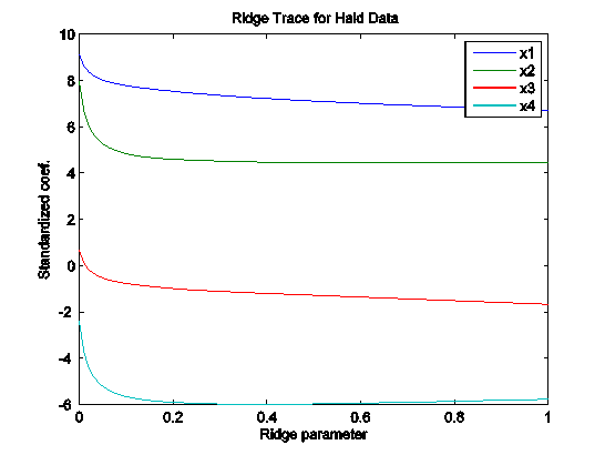
m.ridge <- lm.ridge(lpsa ~ .,data=data.train, lambda = seq(0,20,0.1))
plot(m.ridge)
# select parameter by minimum GCV
plot(m.ridge$GCV)
# Predict is not implemented so we need to do it ourselves
y.pred.ridge = scale(data.test[,1:8],center = F, scale = m.ridge$scales)%*% m.ridge$coef[,which.min(m.ridge$GCV)] + m.ridge$ym
summary((y.pred.ridge – y.test)^2)
####################################
## Lasso
####################################
library(lars)
m.lasso <- lars(as.matrix(data.train[,1:8]),data.train$lpsa)
plot(m.lasso)
# Cross-validation
r <- cv.lars(as.matrix(data.train[,1:8]),data.train$lpsa)
bestfraction <- r$fraction[which.min(r$cv)]
##### Note 5/8/11: in the new lars package 0.9-8, the field r$fraction seems to have been replaced by r$index. The previous line should therefore be replaced by:
# bestfraction <- r$index[which.min(r$cv)]
# Observe coefficients
coef.lasso <- predict(m.lasso,as.matrix(data.test[,1:8]),s=bestfraction,type=”coefficient”,mode=”fraction”)
coef.lasso
# Prediction
y.pred.lasso <- predict(m.lasso,as.matrix(data.test[,1:8]),s=bestfraction,type=”fit”,mode=”fraction”)$fit
summary((y.pred.lasso – y.test)^2)
####################################
## PCR
####################################
library(pls)
m.pcr <- pcr(lpsa ~ .,data=data.train , validation=”CV”)
# select number of components (by CV)
ncomp <- which.min(m.pcr$validation$adj)
# predict
y.pred.pcr <- predict(m.pcr,data.test , ncomp=ncomp)
summary((y.pred.pcr – y.test)^2)
####################################
## PLS
####################################
library(pls)
m.pls <- plsr(lpsa ~ .,data=data.train , validation=”CV”)
# select number of components (by CV)
ncomp <- which.min(m.pls$validation$adj)
# predict
y.pred.pcr <- predict(m.pls,data.test , ncomp=ncomp)
summary((y.pred.pcr – y.test)^2)
%%%%%%%%%%%%%%%%%%%%%%%%%%%%%%%%%%%%%%%%%%
%
% File: Lasso.m
% Author: Jinzhu Jia
%
% One simple (Gradiant Descent) implementation of the Lasso
% The objective function is:
% ۱/۲*sum((Y – X * beta -beta0).^2) + lambda * sum(abs(beta))
% Comparison with CVX code is done
% Reference: To be uploaded
%
% Version 4.23.2010
%%%%%%%%%%%%%%%%%%%%%%%%%%%%%%%%%%%%%%%%%%%%%
function [beta0,beta] = Lasso(X,Y,lambda)
n = size(X,1);
p = size(X,2);
if(size(Y,1) ~= n)
fprintf( ‘Error: dim of X and dim of Y are not match!!\n’)
quit cancel
end
beta0 = 0;
beta= zeros(p,1);
crit = 1;
step = 0;
while(crit > 1E-5)
step = step + 1;
obj_ini = 1/2*sum((Y – X * beta -beta0).^2) + lambda * sum(abs(beta));
beta0 = mean(Y – X*beta);
for(j = 1:p)
a = sum(X(:,j).^2);
b = sum((Y – X*beta).* X(:,j)) + beta(j) * a;
if lambda >= abs(b)
beta(j) = 0;
else
if b>0
beta(j) = (b – lambda) / a;
else
beta(j) = (b+lambda) /a;
end
end
end
obj_now = 1/2*sum((Y – X * beta -beta0).^2) + lambda * sum(abs(beta));
crit = abs(obj_now – obj_ini) / abs(obj_ini);
end
مثال خروجی :